
Through a series of blogs, we will explain the basics of fiber link models and power budgets (the amount of loss a data link can tolerate while maintaining proper operation) using multimode fiber and singlemode fiber.
To understand this, it’s important to start with the basics – which is what we’ll cover here.
Fiber Link Models
The IEEE 802.3 standard refers to the fiber link model as the “fiber optic cabling model.” This model specifies the link characteristics of each element in an optical link: transceiver performance, fiber cable performance and maximum reach, and connector performance and maximum connection loss.
The fiber optic cabling channel contains one or multiple optical fibers for each direction to support an optical link. It interconnects transmitters at the MDI (medium-dependent interface, or the optical interface at the transceiver module that connects to the optical cable connecter).
If the components used in the optical link comply with standard specifications, then we’re assured that we have solid link performance at the Ethernet physical layer: Our data centers and networks run better and faster, with less downtime.
Standard specifications for fiber link performance cover:
- Optical interface (MDI) mechanical specification
- Physical transmission media (OS1/OS2 singlemode or OM1, OM2, OM3, OM4 and OM5 multimode fiber)
- Power budget (the maximum allowed power difference between transmitter power and receiver power in optica modulation amplitude [OMA], i.e. the difference between power for Level 1 and Level 0)
- Power penalty caused by transmission in the fiber and transmitter
- Channel insertion loss (caused by fiber attenuation, specified in dB; the amount of loss a fiber link can tolerate)
- Maximum transmission distance for different fiber types
- Cable performance (cable skew, i.e. transmission time difference between different fibers in the same cable)
- Fiber connector performance (each connector has a maximum insertion loss limit; there’s also a specification for total connector loss)
Correlation Between Fiber Link Models and Power Budgets
As described above, the amount of loss a fiber link can tolerate is referred to as “channel insertion loss.” Power budget and channel insertion loss are not the same.
Power budget = channel insertion loss + allocation for penalties + additional insertion loss allowed
As an example, let’s take a closer look at the 100GBASE-SR4 specification. The allocation for penalties in this example is caused by transmitter and dispersion eye closure (TDEC). Here, the optical eye closes due to noise, jitter and fiber dispersion (optical pulses spreading as they travel down the fiber).
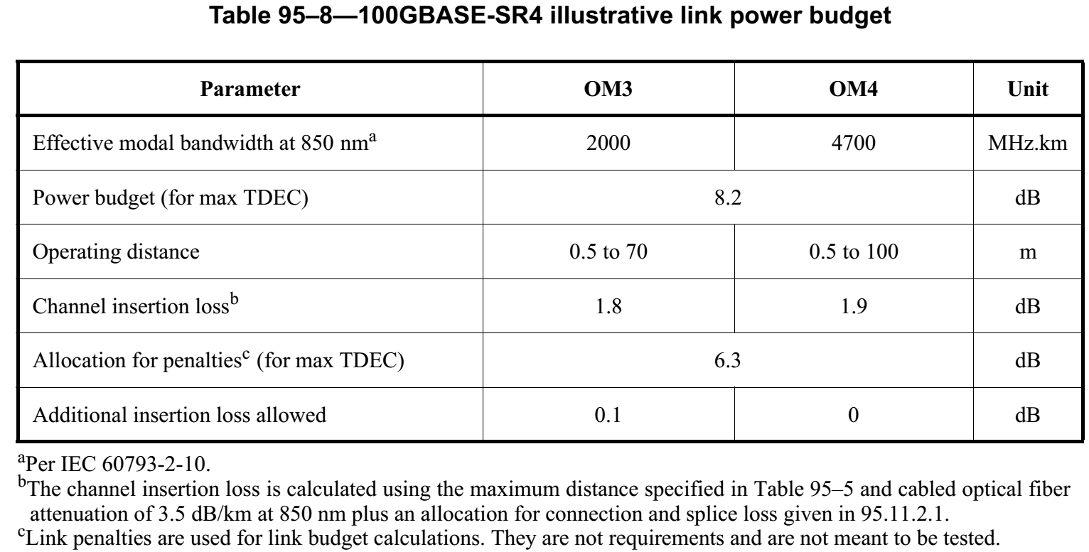
IEEE 802.3 Ethernet Specification for 100GBASE-SR4 Link Power Budget
If you use 100GBASE-SR4 and 100m OM4 fiber cable (multiple sections with connectors) with the transmitter power of 0 dBm in OMA (optical modulation amplitude) and stressed receiver sensitivity of -8.2 dBm (with the worst acceptable signal received), then the power budget is equal to 8.2 dB. Only 1.9 dB is allocated for cable and connector loss; 6.3 dB is allocated for transmission penalty (the signal will be distorted and noisier after 100m transmission).
Why Does This Matter?
When we have multiple points of connection in a structured fiber cabling system, it’s important to know your link model and power budget. As we mentioned earlier, link performance becomes vitally important as data centers migrate to 40G, 100G, 200G and 400G. Dead fiber links cause system downtime (which equates to increased costs, frustrated users and increased total cost of ownership).
Total channel insertion loss must be below the standard specification. In the 100GBASE-SR4 example mentioned above, total channel insertion loss is 1.9 dB. Total insertion allocated for fiber cable is 0.4 dB; the allocation for fiber connections is 1.5 dB. Each connector will contribute no more than 0.75 dB; you can support seven points of connection instead of two if you keep connector loss lower, such as 0.2 dB per connection.
A high-performance link that offers improved return loss requires high-performance cables, quality transceivers and high-performance installation practices.
How Does This Translate to Data Center Performance?
Many data center managers find themselves debating between reusing installed fiber cable and deploying new fiber infrastructure to manage up-and-coming technology. Especially as next-generation speeds impact enterprises, it’s important to make the right decision about fiber optic cabling to futureproof your infrastructure.
Don’t forget that the total cost of ownership makes up more than just the costs of transceivers, cabling and installation – it also involves maintenance costs. High performance cable provides better link performance and more flexible cabling for cross-connects and fiber-use efficiency, which ultimately cuts down on regular maintenance expenses.
When you understand the fiber link budget you have access to (the channel insertion loss), then you can optimize your fiber link design as well. For example, if you use shorter cable runs, then you can create more connection points. If you employ low-loss connectors and low-loss fiber cable, then you can support longer distances.
Working with a high-quality, trusted data center partner can go a long way toward ensuring that you have a futureproof fiber optic system you can afford, and that supports your organization for years to come. To learn more about partnering with Belden for your data center project, visit https://www.belden.com/partners/partner-programs.
About the author
Qing Xu
Technology and Application Manager, Optical Fiber Systems
With 13 years of experience in optical communications and photonics device design, Qing Xu is a subject-matter expert in not only optical fiber technology, but also signal transmission, data center trends, fiber/copper connectivity and structured cabling. During his time with Belden, he closely monitored and participated in industry activities related to optical fiber communications systems, data center technology and trends.